DNA Extraction and B.E.S.T. library construction from Herbarium Ficus leaves

Over the past few weeks, we’ve been experimenting with DNA extraction and Illumina library construction using Ficus herbarium samples. Some of which are a century old. The library preparation follows the B.E.S.T. protocol (Carøe et al., 2018), which is designed for working with degraded DNA such as that found in museum specimens.

For the DNA extractions, we used a modified protocol of the Qiagen DNeasy Plant Mini Kit. A big thank you to the Martin Lab at the NTNU University Museum for sharing their DNA extraction and B.E.S.T. library preparation protocols, which included very helpful tips. We made a slight modification to the BEST library protocol by using NEB Q5U DNA Polymerase for library indexing and amplification. This polymerase does not require an extended warm start and, importantly, does not stall when encountering uracil, a common feature of damaged or degraded DNA resulting from cytosine deamination.

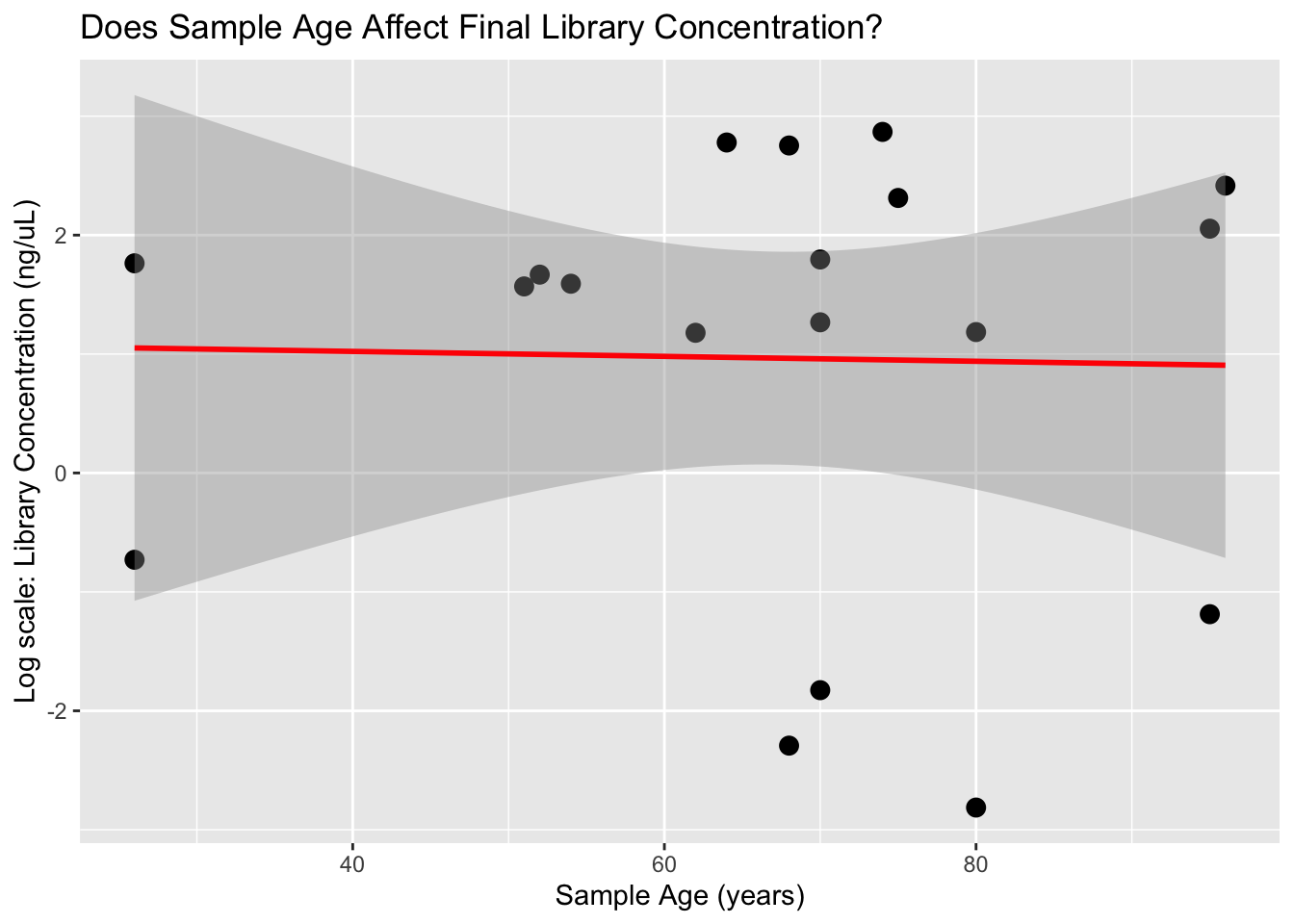
Below, we examine the 20 libraries and the DNA extraction we have performed so far. We aim to investigate whether there are any trends or correlations between DNA concentrations and BEST Library concentrations with respect to sample age. I hope this helps us with future DNA constructions.

Load in Libraries and READ

Code

library("tidyverse")
library("readxl")

Here we are reading in the data for current sample DNA extractions and B.E.S.T. library preparations.

Code

dna <- read_xlsx("DNA_and_BEST_lib.xlsx", sheet="DNA")
lib <- read_xlsx("DNA_and_BEST_lib.xlsx", sheet="Libraries")

#remove last samples since it is a wasp
lib <- lib[-20,]

knitr::kable(dna)

Sample	DNA_conc.	Sample_input	Collection_Year	Locality
FC132.921I	1.30	20.00	1999	Puerto Rico
FC89.921I	1.47	10.00	1955	Haiti
FA20.921I	1.60	10.00	1930	Domiinican Republic
FA59.921I	1.19	10.00	1945	Mexico
FC132.proK.922I	13.00	20.00	1999	Puerto Rico
FC89.proK.922I	1.29	10.00	1955	Haiti
FA20.proK.922I	1.35	10.00	1930	Domiinican Republic
FA59.proK.922I	0.35	7.00	1945	Mexico
FA26.1021I	1.33	11.00	1957	Guadeloupe
FA44.1021I	1.12	11.80	1971	Jamaica
FA45.1021I	1.43	12.10	1963	Jamaica
FA67.1021I	1.64	10.00	1974	Florida
FA68.1021I	39.70	13.40	1961	Florida
FA69.1021I	19.60	17.20	1955	Florida
FA70.1021I	26.00	17.00	1951	Florida
FA73.1021I	7.18	11.20	1950	Florida
FA16.1028I	4.81	10.00	1929	Cuba
FA17.1028I	10.30	13.30	1957	Domiinican Republic
FA63.1028I	1.42	14.40	1973	Nicaragua
FA1.1022I	8.41	13.60	1975	Bahamas
FA2.1022I	11.20	17.10	1967	Bahamas
FA3.1022I	4.22	17.10	1948	Bahamas
FA4.1022I	24.90	15.40	1948	Bahamas
FA12.1022I	8.08	18.80	1994	Cuba
FA15.1022I	33.20	15.40	1941	Cuba
FA71.1022I	9.00	15.00	1950	Florida
FA72.1022I	14.60	16.24	1940	Florida

Code

knitr::kable(lib)

Library ID	Sample	Collection_Year	DNA_conc.	Library Conc.	Cycles
BL1.1022	FC132.ProkI.922	1999	13.00	0.482	5
BL2.1022	FC89.ProkI.922	1955	1.29	0.161	7
BL3.1022	FA20.ProkI.922	1930	1.35	0.305	7
BL4.1022	FA59.ProkI.922	1945	0.35	0.060	7
BL5.1030	FC132.ProkI.922	1999	13.00	5.830	14
BL6.1030	FC89.ProkI.922	1955	1.29	6.020	14
BL7.1030	FA20.ProkI.922	1930	1.35	7.800	14
BL8.1030	FA59.ProkI.922	1945	0.35	3.270	14
BL9.1030	FA26.1021I	1957	1.33	0.101	15
BL10.1030	FA44.1021I	1971	1.12	4.910	15
BL11.1030	FA45.1021I	1963	1.43	3.250	15
BL12.1030	FA67.1021I	1974	1.64	4.800	15
BL13.1030	FA68.1021I	1961	39.70	16.100	15
BL14.1030	FA69.1021I	1955	19.60	3.550	15
BL15.1030	FA70.1021I	1951	26.00	17.600	15
BL16.1030	FA73.1021I	1950	7.18	10.100	15
BL17.1030	FA16.1021I	1929	4.81	11.200	15
BL18.1030	FA17.1021I	1957	10.30	15.700	15
BL19.1030	FA63.1021I	1973	1.42	5.300	15

Explorative Statistics

Code

# Compute sample age (if not included)
dna <- dna %>%
  mutate(SampleAge = 2025 - Collection_Year)

lib <- lib %>%
    mutate(SampleAge = 2025 - Collection_Year,
    DNA_input = DNA_conc. * 16)

Summary Statistic for DNA Extractions

Code

summary(dna)

    Sample            DNA_conc.       Sample_input   Collection_Year
 Length:27          Min.   : 0.350   Min.   : 7.00   Min.   :1929   
 Class :character   1st Qu.: 1.385   1st Qu.:10.00   1st Qu.:1946   
 Mode  :character   Median : 4.810   Median :13.40   Median :1955   
                    Mean   : 9.248   Mean   :13.59   Mean   :1958   
                    3rd Qu.:12.100   3rd Qu.:16.62   3rd Qu.:1969   
                    Max.   :39.700   Max.   :20.00   Max.   :1999   
   Locality           SampleAge    
 Length:27          Min.   :26.00  
 Class :character   1st Qu.:56.00  
 Mode  :character   Median :70.00  
                    Mean   :67.15  
                    3rd Qu.:78.50  
                    Max.   :96.00

Code

dna %>% summarise(across(where(is.numeric), mean, na.rm = TRUE))

Warning: There was 1 warning in `summarise()`.
i In argument: `across(where(is.numeric), mean, na.rm = TRUE)`.
Caused by warning:
! The `...` argument of `across()` is deprecated as of dplyr 1.1.0.
Supply arguments directly to `.fns` through an anonymous function instead.

  # Previously
  across(a:b, mean, na.rm = TRUE)

  # Now
  across(a:b, \(x) mean(x, na.rm = TRUE))

# A tibble: 1 x 4
  DNA_conc. Sample_input Collection_Year SampleAge
      <dbl>        <dbl>           <dbl>     <dbl>
1      9.25         13.6           1958.      67.1

Summary Statistic for Library Preparation

Code

summary(lib)

  Library ID           Sample          Collection_Year   DNA_conc.     
 Length:19          Length:19          Min.   :1929    Min.   : 0.350  
 Class :character   Class :character   1st Qu.:1948    1st Qu.: 1.310  
 Mode  :character   Mode  :character   Median :1955    Median : 1.430  
                                       Mean   :1958    Mean   : 7.711  
                                       3rd Qu.:1967    3rd Qu.:11.650  
                                       Max.   :1999    Max.   :39.700  
 Library Conc.        Cycles     SampleAge       DNA_input     
 Min.   : 0.060   Min.   : 5   Min.   :26.00   Min.   :  5.60  
 1st Qu.: 1.866   1st Qu.:14   1st Qu.:58.00   1st Qu.: 20.96  
 Median : 4.910   Median :15   Median :70.00   Median : 22.88  
 Mean   : 6.134   Mean   :13   Mean   :67.16   Mean   :123.38  
 3rd Qu.: 8.950   3rd Qu.:15   3rd Qu.:77.50   3rd Qu.:186.40  
 Max.   :17.600   Max.   :15   Max.   :96.00   Max.   :635.20

Code

lib %>% summarise(across(where(is.numeric), mean, na.rm = TRUE))

# A tibble: 1 x 6
  Collection_Year DNA_conc. `Library Conc.` Cycles SampleAge DNA_input
            <dbl>     <dbl>           <dbl>  <dbl>     <dbl>     <dbl>
1           1958.      7.71            6.13     13      67.2      123.

Correlation between variables

Code

cor(dna$SampleAge, dna$DNA_conc., use = "complete.obs")

[1] 0.07591351

Code

cor(dna$Sample_input, dna$DNA_conc., use = "complete.obs")

[1] 0.4233805

Code

cor(lib$DNA_input, lib$`Library Conc.`, use = "complete.obs")

[1] 0.6343754

Code

cor(lib$Cycles, lib$`Library Conc.`, use = "complete.obs")

[1] 0.5686558

Code

cor(lib$SampleAge, lib$`Library Conc.`, use = "complete.obs")

[1] 0.142088

Visualization

Here we are plotting some of our variable to visualize trends

Older samples yield less DNA?

Code

ggplot(dna, aes(x = SampleAge, y = DNA_conc.)) +
  geom_point(size = 3) +
  geom_smooth(method = "lm", se = TRUE, color = "blue") +
  labs(x = "Sample Age (years)", y = "DNA Extraction Concentration (ng/µL)",
       title = "Older samples yield less DNA?")

`geom_smooth()` using formula = 'y ~ x'

Does input mass affect DNA yield?

Code

ggplot(dna, aes(x = Sample_input, y = DNA_conc.)) +
  geom_point(size = 3) +
  geom_smooth(method = "lm", se = TRUE, color = "blue") +
  labs(x = "Input Sample Mass (mg)", y = "DNA Extraction Concentration (ng/µL)",
  title = "Does input mass affect DNA yield?")

`geom_smooth()` using formula = 'y ~ x'

Does DNA input mass affect final Library Concentration?

Code

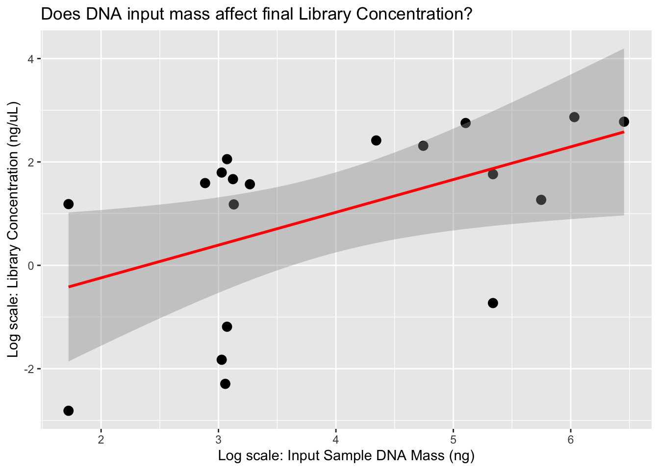
ggplot(lib, aes(x = log(DNA_input), y = log(`Library Conc.`))) +
  geom_point(size = 3) +
  geom_smooth(method = "lm", se = TRUE, color = "red") +
  labs(x = "Log scale: Input Sample DNA Mass (ng)", y = "Log scale: Library Concentration (ng/µL)",
  title = "Does DNA input mass affect final Library Concentration?")

`geom_smooth()` using formula = 'y ~ x'

Does Sample Age Affect Final Library Concentration?

Code

ggplot(lib, aes(x = SampleAge, y = log(`Library Conc.`))) +
  geom_point(size = 3) +
  geom_smooth(method = "lm", se = TRUE, color = "red") +
  labs(x = "Sample Age (years)", y = "Log scale: Library Concentration (ng/µL)",
  title = "Does Sample Age Affect Final Library Concentration?")

`geom_smooth()` using formula = 'y ~ x'

PCR Cycles and Library Concentration

Code

ggplot(lib, aes(x = factor(Cycles), y = `Library Conc.`)) +
  geom_boxplot(fill = "steelblue", alpha = 0.7) +
  geom_jitter(width = 0.2, alpha = 0.6) +
  labs(x = "PCR Cycles",
       y = "Library Concentration (ng/µL)",
       title = "Variation in Library Yield Across PCR Cycle Counts") +
  theme_minimal()

Conclusion

It appears that the DNA input mass is the primary factor influencing the amount of DNA recovered during the extraction process. Based on these results, we’ll aim for at least 10 mg of tissue per extraction to ensure we have sufficient material for downstream steps. Currently, we’re eluting in 62 µL, but we plan to reduce this to 50 µL to enhance DNA concentration and increase the total DNA input into our BEST library prep (we use 16 µL of extract per reaction). This is a minor modification from the Martin Lab protocol, as we’re performing half-volume reactions to reduce reagent usage and allow more library constructions.

Our next step will be to run a test sequencing batch to evaluate how these libraries perform. We didn’t include a size selection step, so we expect a higher number of short insert-size fragments. However, we did perform a 1:1 SPRI bead cleanup after PCR, which should have removed most fragments (plus the 132 bp adapters) below ~200 bp, meaning the shortest insert sizes should be around 70 bp.

We ran an agarose gel on an aliquot of our library to assess the distribution of fragment sizes. Most fragments were approximately 300 bp in length, corresponding to an insert size of around 168 bp. This is on the shorter side for Illumina libraries and is not ideal; however, they still can be used for variant calling. The biggest issues would be inflated duplicate rates, as two reads might map to the exact same location.

One way to improve the fragment size distribution would be to perform size selection before library indexing and amplification. However, this could significantly reduce the total amount of DNA available for library amplification, which is one of the advantages of the BEST library protocol compared to standard Illumina library prep. Another option is to perform size selection after library amplification, but this would not eliminate the PCR bias, particularly the overrepresentation of shorter fragments.

Another challenge we are currently seeing is that some libraries have very low concentrations, around 3 ng/µL. If this is due to an excess of smaller fragments, it remains a concern. Increasing PCR cycles may boost yield, but this approach can also increase duplication rates, thereby reducing library complexity.